semopy

Random effects

In many cases researcher must take population structure into an account. Presence of such a structure can be rephrased as a presence of autocorrelation in the data, i.e. observations are not inpedendent. Other popular notions of population structures are grouped, clustered data.

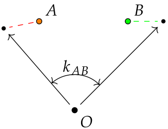
One way to interpret this dependence is to assume that there is an unique additive vector per each group (a "group mean"):

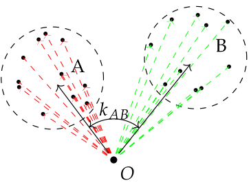
Sample of points from groups A and B. Dashed arrows of red and blue colours are unknown per individual shifts caused by random effect for groups A and B respectively. Black arrows are estimators for random effects of groups. Presence of an apriori information on the angle between mean vectors is helpful, but not neccessary in cases of multiple individuals per group.

In mixed models theory, random effects are not really estimated, but instead they represent random variables, usually normally distributed, that make impact on variance components estimates.

Naive across-group centering

Given interpetation of random effects above, in case of multiple individuals pre group, group-wise means can be a good estimator of random effects. In fact, fitting model to data centered with respect to groups is the same as fitting the model to within-covariance matrix.

Although quiet straightforward in terms of implementation, semopy can do group-wise centering automatically on user's command by supplying a groups argument with list of group names (data columns) to center across to the fit method. For instance, let's assume a toy example of multivariate regression model and let's add random noise across 3 groups to the dataset:

from semopy.examples import multivariate_regression
from semopy import ModelMeans

desc = multivariate_regression.get_model()
data = multivariate_regression.get_data()
data['group'] = 0
np.random.seed(10)
U =  np.array([np.random.normal(scale=1, size=1).flatten() for _ in range(3)])
data.iloc[0:25, 3] +=  U[0].flatten()
data.iloc[0:25, -1] = 0
data.iloc[25:50, 3] += U[1].flatten()
data.iloc[25:50, -1] = 1
data.iloc[50:75, 3] +=  U[2].flatten()
data.iloc[50:75, -1] = 2

mod = ModelMeans(desc)
mod.fit(data, groups=['group'])
print(mod.inspect())

Output:

lval  op rval   Estimate  Std. Err     z-value       p-value
   y   ~   x1   1.993463  0.134835   14.784412  0.000000e+00
   y   ~   x2   6.002902  0.038818  154.642088  0.000000e+00
   y   ~   x3  -9.968743  0.247988  -40.198442  0.000000e+00
   y   ~    1 -54.613792  0.421791 -129.480835  0.000000e+00
   y  ~~    y   5.702523  0.806459    7.071068  1.537437e-12

• Impossible to apply in case of group size 1, i.e. when individual observations themselves are not independent;
• Information on intercepts is lost irreversibly (notice the mean component above);
• Between-groups variance is not analysed.

Model with random effects

semopy provides a generalization of classical Linear Mixed Models to SEM. Random effects model resides in ModelEffects class. It's evaluated in the same fashion as Model or ModelMeans classes, the only difference is that there is one extra mandatory and one optional arguments to the fit method:

1. group: a name of group mapping column in a dataset (mandatory);
2. k: covariance across groups matrix (also known as genetic kinship matrix in genomic studies) (optional, the default is identity matrix).

m = ModelEffects(mod)
m.fit(data, group='group')
print(m.inspect())

lval     op rval  Estimate Std. Err  z-value   p-value
   y      ~   x1  1.92960  0.06194   31.15294  0.00000
   y      ~   x2  6.03267  0.01786  337.72220  0.00000
   y      ~   x3 -9.74500  0.11431  -85.25059  0.00000
   y      ~    1 -0.36861  0.89062   -0.41388  0.67895
   y     ~~    y  0.00000  1.08692    0.00000  1.00000
   y     RF    y  2.26582  1.63066    1.38951  0.16467
   1  RF(v)    1  1.19841  0.12360    9.69536  0.00000

However, if the user is interested in analysying variances, it might be more difficult for him/her to interpret the estimates of variances produced by ModelEffects. Here, RF operator stands for variances of random effects themselves. More elaborate explanation is available in the Matrices and variables section. It's often the case that it is hard for the optimizer to properly separate variable's variance from variance that is introduced to them by a population structure. Sometimes this problem arises even in the simple examples as the one above. In such cases, variances are usually dispersed across RF and "~~" parameters and should be approached carefully.

Example with correlated individuals

A case of non-independent observations can be thought as a data with population structure, where each individual reside in a group of size 1. That's it, for each observation there is an unique vector that causes some "group-specific" shift to the observation.

In general case, there is no way we can extract those random effect vectors from the data. However, if we have information on the angle between those vectors, or cosines, it might be possible to control for them. Elements of K matrix are essentialy something that is proportianl those cosines. How K is obtained is up to a researcher, however. In case of genomic studies, it is usually computed from genetic markers. In timeseries analysis, it can be a model matrix that assumes certain time-based dependence model.

semopy has a built-in example with data already "polluted" with random effects:

eta1 =~ y1 + y2
eta2 =~ y3 + y4
x2 ~ eta1
eta2 ~ eta1
x1 ~ eta1

Let's evaluate it in semopy:

from semopy.examples import example_rf

desc = example_rf.get_model()
data, k = example_rf.get_data()

model = ModelEffects(desc)
model.fit(data, group='group', k=k)
print(model.inspect())

Output:

 lval     op  rval      Estimate    Std. Err      z-value      p-value
 eta2      ~  eta1  2.928235e+00    0.242339      12.0832            0
   y1      ~  eta1  1.000000e+00           -            -            -
   y2      ~  eta1  3.057422e+00    0.250973      12.1823            0
   y3      ~  eta2  1.000000e+00           -            -            -
   y4      ~  eta2 -1.266143e+00   0.0469064      -26.993            0
   x2      ~  eta1  2.119686e+00    0.183198      11.5705            0
   x1      ~  eta1 -2.356136e+00    0.203165     -11.5972            0
   x2      ~     1  2.935724e-01     82.0531   0.00357783     0.997145
   x1      ~     1 -4.083042e-01     90.6129  -0.00450603     0.996405
   y1      ~     1  2.444895e-01     42.7387   0.00572057     0.995436
   y2      ~     1  5.349159e-01     116.216   0.00460276     0.996328
   y3      ~     1  4.257485e-01     111.588   0.00381535     0.996956
   y4      ~     1 -8.945790e-01     140.626  -0.00636141     0.994924
 eta2     ~~  eta2  4.083493e-15     91.2585  4.47464e-17            1
 eta1     ~~  eta1  1.423499e+03     820.457      1.73501    0.0827394
   x2     ~~    x2  4.023687e+02      265.36      1.51632      0.12944
   y4     ~~    y4  3.156232e-15     357.139  8.83753e-18            1
   y3     ~~    y3  3.610053e+02     278.276      1.29729     0.194531
   x1     ~~    x1  1.818671e+02     271.259     0.670455     0.502568
   y1     ~~    y1  4.254358e+02       250.9      1.69564    0.0899541
   y2     ~~    y2  3.225779e+02      263.39      1.22472     0.220682
   x1     RF    x1  8.680546e-01    0.108888      7.97201  1.55431e-15
   x2     RF    x2  1.421993e-01   0.0161379      8.81154            0
   y1     RF    y1  4.443532e-08  0.00552006  8.04979e-06     0.999994
   y2     RF    y2  3.458323e-01   0.0404847       8.5423            0
   y3     RF    y3  3.111291e-01   0.0362367      8.58603            0
   y4     RF    y4  1.814732e+00    0.250854      7.23422  4.68292e-13
    1  RF(v)     1  9.631969e+00    0.685242      14.0563            0

Those estimates are in agreement with a correct parameter estimates (see example_rf docstring).