semopy

Visualization

semopy provides with a wrapper around graphviz package to quickly plot SEM models. User can visualize his Model instance via call to the semplot function with the following arguments of interest:

1. mod — semopy Model instance;
2. filename — name of file where to plot is saved;
3. plot_covs — If True, covariances are also drawn. The default is False;
4. plot_exos — If False, exogenous variables are not plotted. It might be useful, for example, in GWAS setting, where a number of exogenous variables, i.e. genetic markers, is oblivious. Has effect only with ModelMeans or ModelEffects. The default is True.
5. images — node labels can be replaced with images. It will be the case if a map variable_name->path_to_image is provided.

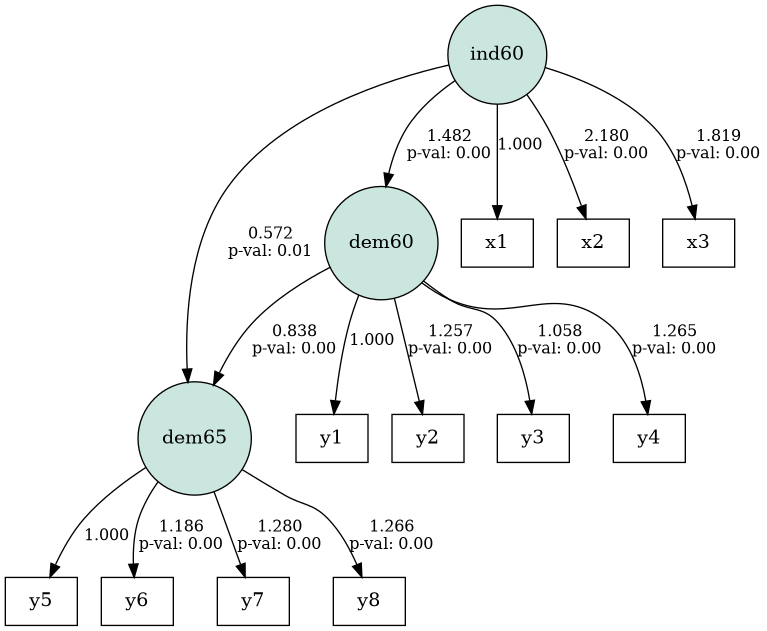
Example:

import semopy

data = semopy.examples.political_democracy.get_data()
mod = semopy.examples.political_democracy.get_model()
m = semopy.Model(mod)
m.fit(data)
g = semopy.semplot(m, "pd.png")

Result:

It's possible to adjust the graphviz graph manually in the "dot"-format as returned by semplot. See:

print(g)

Output:

digraph G {
	overlap=scale splines=true
	edge [fontsize=12]
	node [fillcolor="#cae6df" shape=circle style=filled]
	dem65 [label=dem65]
	ind60 [label=ind60]
	dem60 [label=dem60]
	node [shape=box style=""]
	x1 [label=x1]
	x2 [label=x2]
	x3 [label=x3]
	y1 [label=y1]
	y2 [label=y2]
	y3 [label=y3]
	y4 [label=y4]
	y5 [label=y5]
	y6 [label=y6]
	y7 [label=y7]
	y8 [label=y8]
	ind60 -> dem60 [label="1.482
p-val: 0.00"]
	ind60 -> dem65 [label="0.572
p-val: 0.01"]
	dem60 -> dem65 [label="0.838
p-val: 0.00"]
	ind60 -> x1 [label=1.000]
	ind60 -> x2 [label="2.180
p-val: 0.00"]
	ind60 -> x3 [label="1.819
p-val: 0.00"]
	dem60 -> y1 [label=1.000]
	dem60 -> y2 [label="1.257
p-val: 0.00"]
	dem60 -> y3 [label="1.058
p-val: 0.00"]
	dem60 -> y4 [label="1.265
p-val: 0.00"]
	dem65 -> y5 [label=1.000]
	dem65 -> y6 [label="1.186
p-val: 0.00"]
	dem65 -> y7 [label="1.280
p-val: 0.00"]
	dem65 -> y8 [label="1.266
p-val: 0.00"]
}